
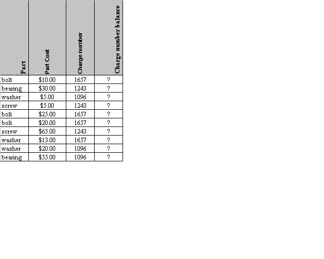
I've included a screen shot of the basic format of the spreadsheet.

Function with filter in excel?
Started by
keepviper13
, Jun 29 2005 12:46 PM
#1

 Posted 29 June 2005 - 12:46 PM
keepviper13
-
- Member
-

- 7 posts
New Member
I've included a screen shot of the basic format of the spreadsheet.

#2
Posted 30 June 2005 - 11:45 AM
keepviper13
- Topic Starter
-
- Member
-
- 7 posts
New Member
somebody have an idea of where to start?
I am pretty confident with a direction i could run with it and figure it out, but i really don't know which functions to try and manipulate to get it to work...
I am pretty confident with a direction i could run with it and figure it out, but i really don't know which functions to try and manipulate to get it to work...
#3
Posted 30 June 2005 - 02:28 PM
keepviper13
- Topic Starter
-
- Member
-
- 7 posts
New Member
............(A).......... ...(B)...............( C )................(D)
1..........Part #..........Price...........Charge #........ Balance
2........1234AA.........22.00..........3AJ123.............?
3........2345AA.........100.00........3AJ123.............?
4........1234AA.........89.00..........4AJ234.............?
5........5678AA.........50.00..........5AA123.............?
6........7890AB.........79.99..........6AC234.............?
7........5678AA.........5.89............4AJ234.............?
8........3456AB.........64.45..........4AJ234.............?
9........1234AB.........234.00........5AA123.............?
10......4567AA.........55.99..........6AC234.............?
Okay, so here is an example....
I am writing the function to return the value in the balance column (D). I want the value in cell D2 to be the spent sum for the charge # in the same row. Therefore, the function must recognize the charge # in that row, then find rows that use the same charge #, then sum the price values of all those rows and report it to the original cell D2. And hopefully that function can be copied down the column to do that over and over for each row.
The completed formula should make the sheet look like so....
............(A)........... ..(B)...............( C )................(D)
1..........Part #..........Price...........Charge #........ Balance
2........1234AA.........22.00..........3AJ123..............122.00
3........2345AA.........100.00........3AJ123..............122.00
4........1234AA.........89.00..........4AJ234..............159.34
5........5678AA.........50.00..........5AA123..............284.00
6........7890AB.........79.99..........6AC234..............135.98
7........5678AA.........5.89............4AJ234..............159.34
8........3456AB.........64.45..........4AJ234..............159.34
9........1234AB.........234.00........5AA123..............284.00
10......4567AA.........55.99..........6AC234..............135.98
Part # is irrelevant when it comes to sorting out...
The balance column is the balance spent on the charge # in the corresponding row, not a running balance down the sheet
And hopefully as i add new lines the formula can just be copied down and will update the balance if another row is added with the same charge #
1..........Part #..........Price...........Charge #........ Balance
2........1234AA.........22.00..........3AJ123.............?
3........2345AA.........100.00........3AJ123.............?
4........1234AA.........89.00..........4AJ234.............?
5........5678AA.........50.00..........5AA123.............?
6........7890AB.........79.99..........6AC234.............?
7........5678AA.........5.89............4AJ234.............?
8........3456AB.........64.45..........4AJ234.............?
9........1234AB.........234.00........5AA123.............?
10......4567AA.........55.99..........6AC234.............?
Okay, so here is an example....
I am writing the function to return the value in the balance column (D). I want the value in cell D2 to be the spent sum for the charge # in the same row. Therefore, the function must recognize the charge # in that row, then find rows that use the same charge #, then sum the price values of all those rows and report it to the original cell D2. And hopefully that function can be copied down the column to do that over and over for each row.
The completed formula should make the sheet look like so....
............(A)........... ..(B)...............( C )................(D)
1..........Part #..........Price...........Charge #........ Balance
2........1234AA.........22.00..........3AJ123..............122.00
3........2345AA.........100.00........3AJ123..............122.00
4........1234AA.........89.00..........4AJ234..............159.34
5........5678AA.........50.00..........5AA123..............284.00
6........7890AB.........79.99..........6AC234..............135.98
7........5678AA.........5.89............4AJ234..............159.34
8........3456AB.........64.45..........4AJ234..............159.34
9........1234AB.........234.00........5AA123..............284.00
10......4567AA.........55.99..........6AC234..............135.98
Part # is irrelevant when it comes to sorting out...
The balance column is the balance spent on the charge # in the corresponding row, not a running balance down the sheet
And hopefully as i add new lines the formula can just be copied down and will update the balance if another row is added with the same charge #
#4
Posted 30 June 2005 - 02:55 PM
keepviper13
- Topic Starter
-
- Member
-
- 7 posts
New Member
SUMIF(range,criteria,[sum criteria])
This works...but... i'd have to type in each charge# in each row for the criteria because it will not just pull the value from the cell if i put the cell reference for criteria.
Is there a way to make the criteria a cell reference?
This works...but... i'd have to type in each charge# in each row for the criteria because it will not just pull the value from the cell if i put the cell reference for criteria.
Is there a way to make the criteria a cell reference?

#6
Posted 03 July 2005 - 06:40 AM
dsm
-

- Member
-
- 98 posts
Member
I am not sure which function would work best, however I tested an alternative approach.
1. Create a pivot table which sums the total for each charge code.
2. Use a Vlookup function to look at the pivot table and display the balance of each charge code.
Only issue is refreshing the pivot table automatically.
1. Create a pivot table which sums the total for each charge code.
2. Use a Vlookup function to look at the pivot table and display the balance of each charge code.
Only issue is refreshing the pivot table automatically.
#7
Posted 08 July 2005 - 12:51 PM
jasonharrod
-

- Member
-
- 18 posts
Member
Try this formula listed in cell d2 and copy it down, it should work for you.
Part Part Cost Charge Number Charge Number Balance
Bolt 10 1657 =SUMIF($C$2:$C$11,"="&C2,$B$2:$B$11)
Bearing 30 1243 100
Washer 5 1096 80
Screw 5 1243 70
Bolt 25 1657 58
Bolt 20 1657 33
Screw 65 1243 65
Washer 13 1657 13
Washer 20 1096 75
Bearing 55 1096 55
^^ BAD DATA, check my last post
Part Part Cost Charge Number Charge Number Balance
Bolt 10 1657 =SUMIF($C$2:$C$11,"="&C2,$B$2:$B$11)
Bearing 30 1243 100
Washer 5 1096 80
Screw 5 1243 70
Bolt 25 1657 58
Bolt 20 1657 33
Screw 65 1243 65
Washer 13 1657 13
Washer 20 1096 75
Bearing 55 1096 55
^^ BAD DATA, check my last post
Edited by jasonharrod, 10 July 2005 - 09:33 PM.
#8
Posted 09 July 2005 - 10:31 AM
Chronos0001
-

- Member
-
- 43 posts
Member
OK, it looks to me as if you need a little organization. Soooo..
Copy the entire spreadsheet and "paste Special" to another sheet in your workbook. Then on that other sheet "sort" them according to the charge number (make sure you select all of the colums when you sort) After you have sorted, then choose a random cell to sum your charge numbers. Do this for each charge number.
After you have those sums, then "paste special" those cell values back to your original spreadsheet.
What this does, is take any value that you input on the original, automatically updates the second spreadsheet, totals the values, and brings back the updated values from the charges in different locations to a single point. Using the second sheet maintains the integrety of your original format.
Using the summed values that you are bringing back can also help you in creating graphs which will aid you in knowing at a glance which account is the most active, or what parts account (by charge) needs to be re-ordered.. use your imagination
At least that is what I understood from your original request. Unless you are looking to query your database of parts, then you might want to look at using Access to manipulate your data.
Hope that helped.
#9
Posted 09 July 2005 - 10:55 AM
Chronos0001
-
- Member
-
- 43 posts
Member
I took another look at your spreadsheet, trying to figure out what your are trying to sum....
I think you are not concerned about the number of charge accounts, but the number (or balance) of items on those accounts. So...
I built a small spread sheet based on the numbers provided in your sample.
It is in the attachment (if I can send it correctly) (if I can't then contact me directly at my member name @hotmail.com)
I can not send an .xls document over this server, so contact me at the addy provided and I will email it to you.
You will see that on the second page of the spreadsheet I sorted the different accounts by number. This brought all of the balances of the parts in the same charge numbers together and I summed those values.
I then "paste link" that sum to the front page.
Good luck
#10
Posted 10 July 2005 - 09:11 PM
jasonharrod
-
- Member
-
- 18 posts
Member
Use this formula in D2 and copy it down.
=SUMIF($C$2:$C$11,"="&C2,$B$2:$B$11)
Here is the logic behind the formula
basically if any thing in the range of data in COlumn C is equal to the current "charge acc." cell that you want the value in. (Which is D2) Sum up all price in the B Column range and return the value to the current cell.
I'll take this a step further to make your project maintenance free. The following formula when copied from cell D2 all the way to the end of the spreadsheet D65XXX, will return nothing if there is nothing (No #N/A errors) in cell B(CurrentRow()); otherwise it will return the Total for that account.
=IF(B2="","",SUMIF(C:C,"="&C2,B:B))
This I believe is what you are looking for.
These are my results.
PART ... Price.... Charge Ac. TOTAL
Bearing... 30... 1243... 100
Washer... 5... 1096... 80
Screw... 5... 1243... 100
Bolt... 25... 1657... 58
Bolt... 20... 1657... 58
Screw... 65... 1243... 100
Washer... 13... 1657... 58
Washer... 20... 1096... 80
Bearing... 55... 1096... 80
Edited by jasonharrod, 10 July 2005 - 09:32 PM.
#11
Posted 11 July 2005 - 06:34 AM
keepviper13
- Topic Starter
-
- Member
-
- 7 posts
New Member
Works great, i used the sumif function, thanks for the help


Similar Topics
0 user(s) are reading this topic
0 members, 0 guests, 0 anonymous users
As Featured On:


 Sign In
 Create Account
